


Quick answer
In 100,000 simulated experiments with no effect, a two-sided 5% test flagged 4.90% of runs at one final check. Reusing the same threshold at up to 20 cumulative checks flagged 24.63%. Dividing the 5% budget across 20 preplanned checks flagged 1.833% under this model.
Take Rate null simulation; sequential inference background from Johari et al.
Key findings and sources
One final check versus twenty ordinary checks
In Take Rate’s simulation of 100,000 no-effect experiments with cumulative Gaussian data, a two-sided 5% test flagged 4.90% of runs at one final check and 24.63% when reused at up to 20 checks. This is a simulated error rate under the stated model.
Take Rate null simulation; sequential inference background from Johari et al.
Four and ten planned chances to act
In the same 100,000-path Take Rate null simulation, ordinary two-sided 5% tests flagged at least once in 12.659% of runs with four cumulative checks and 19.361% with ten. The schedules reused data and ended at the same information step.
Take Rate null simulation; sequential inference background from Johari et al.
The effect of allocating the error budget in advance
In Take Rate’s 20-check null simulation, a two-sided per-check threshold of 0.25% flagged 1.833% of 100,000 runs, compared with 24.63% when applying 5% at each check. The adjustment trades away sensitivity and the result is specific to the simulated model.
Take Rate null simulation; sequential inference background from Johari et al.
A fixed-horizon test and continuous monitoring require different inference
Johari et al. describe always-valid inference methods for A/B tests in which analysts may choose when to stop based on the observed data. Take Rate’s simulation illustrates why repeated use of an ordinary fixed-horizon threshold changes its error behavior.
Take Rate null simulation; sequential inference background from Johari et al.
Three independent final tests can produce at least one false alarm
In an illustrative no-effect calculation with three independent 5% tests and one final read per outcome, the chance that at least one test flags is 14.26%. Correlated merchant outcomes can give a different result.
Take Rate null simulation; sequential inference background from Johari et al.
Four in five paths that ever flagged were clear at the final look
In Take Rate’s seeded 100,000-path null simulation, 19,730 of 24,630 paths that crossed the ordinary threshold at least once were below it at the final look (80.11%).
Take Rate null simulation; sequential inference background from Johari et al.
Original Take Rate replay using 20 equal information increments and a fixed two-sided 5% threshold. Count ever-flagged paths with a nonflagged final look and divide by all ever-flagged paths.
The first five looks produced 56.37% of first flags
In the same simulated null paths, 13,884 of the 24,630 paths that ever flagged first crossed at looks one to five, or 56.37%. This is a simulation result for the stated information schedule.
Take Rate null simulation; sequential inference background from Johari et al.
Same seeded 100,000 independent null paths and ordinary threshold. Count the first crossing location for each flagged path and divide the first-five count by ever-flagged paths.
Compare the results
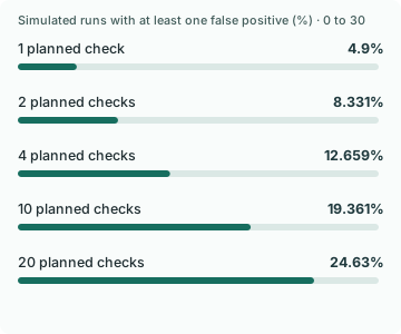
One final test and twenty opportunities answer different questions
Under the null simulation, one final check flagged 4,900 of 100,000 paths. Two checks flagged 8,331, four flagged 12,659, ten flagged 19,361 and twenty flagged 24,630. The displayed rate is the share of runs with at least one two-sided flag. It does not count how many flags appeared inside an individual run.
Every schedule uses the same generated paths and the same final information step. The difference is the number of times the team could act on a crossing. Cumulative measurements reuse earlier observations, so the checks are correlated. Treating them as independent and calculating one minus 0.95 raised to the number of checks would answer a different question.
If you choose to report the first positive result, the chance of reporting a false positive no longer has the same interpretation as a single final test. The same problem applies if you stop at a negative crossing or choose which day to show after reading the result. The decision rule is part of the statistical design.
A preplanned correction cuts false alarms and trades away sensitivity
The simulation also divides the 5% family error budget by the number of planned checks. That gives a two-sided threshold of 0.25% at each of 20 checks. Under the same null paths, 1,833 runs flagged at least once, or 1.833%. The correction is conservative because the cumulative checks are correlated.
A lower null flag rate by itself does not make the plan better. A stricter threshold can make a real gain harder to detect. If early action is valuable, choose a properly calibrated sequential design rather than repeatedly applying an ordinary fixed-horizon threshold. Johari and colleagues describe inference procedures designed for continuous monitoring.
Pick the primary business outcome and the measurement window. Then decide whether you need one final decision, a small set of prespecified looks or a sequential rule. Set the stopping criteria before opening the first result and keep the original assignments if you investigate delivery, returns or exposure later.
Separate safety monitoring from claiming a positive effect
A checkout team may need to stop quickly when a payment route fails or a confirmation message sends twice. Operational monitoring has a different purpose from claiming that a tested change improved conversion. Define the safety rule, record why the test stopped and use an inference procedure that reflects the actual plan if you report effect estimates.
Checking conversion, gross sales, net contribution and refunds for any favorable p-value creates a second selection opportunity. This simulation varies the number of time checks for one outcome only. It does not estimate the joint false-positive rate when teams also try multiple metrics, audiences or attribution windows.
For a decision record, keep the assigned counts, data cutoff, primary outcome and test rule next to the estimate. If a promising exploratory metric appeared after the fact, use it to write a new hypothesis. The next test can make that metric a planned decision instead of retroactively treating it as the original one.
How to replay the calculation and where it stops applying
The downloadable Python file generates 20 independent standard-normal increments for each path. At time t it divides their cumulative sum by the square root of t and compares the absolute value with the two-sided critical threshold. The seed, increments, schedules, thresholds and exact flag counts are recorded in the output.
This model has no true effect, known variance and evenly spaced information steps. A merchant’s experiment can have uneven traffic, repeat visits, revenue outliers or delayed refunds. Those conditions change the design and can change the false-positive behavior. The simulation makes the repeated-look effect reproducible without estimating any store’s result.
A single readout can still offer several chances to declare a win
Waiting until the final day solves the repeated-look problem for a single prechosen outcome. A team that calls a test successful when any of checkout conversion, order revenue or gross margin improves still gives itself several chances. The outcomes may be correlated because they come from the same customers.
If three no-effect outcomes were independent and each used a single two-sided 5% test, the chance of at least one flag would be 14.26%. If each independent outcome instead had the 24.63% flag rate of the 20-look schedule in this simulation, the worked calculation gives about 57.19%. Both are examples under an independence assumption. They do not estimate the error rate for three correlated merchant metrics.
Choose which outcome decides the test and list the others as diagnostic or safety measures. If several metrics truly can justify a win, set the joint testing rule before collecting the results. A team can still investigate secondary effects after the experiment, then confirm them in a fresh test before making a rollout claim.
Most paths flagged early eventually failed the final threshold
Among the 24,630 paths that crossed the ordinary threshold at any of 20 looks, 19,730 ended below the threshold at the final look. That is 80.11% of the paths that had signaled at least once. Every path comes from the same no-effect data model and uses the same fixed critical value at every look. Following those exact paths to the final point isolates the disagreement between an early claim and a final readout.
The timing distribution also matters. First flags in the first five looks accounted for 56.37% of all flagged paths, while 2,250 paths first crossed in the last five looks. In these paths the looks are equally spaced in information. The shape can differ when a merchant uses uneven calendar cuts, a minimum sample guard, or a noisier revenue outcome.
Write down which early observations can change the experiment
A team should be able to stop for a payment outage, a broken assignment rule or a severe customer harm signal. Those are safety and operations decisions. They can be logged independently of a rule for declaring that a treatment increased sales. Define which events permit a stop and what result can be stated after one.
If you need to act on evidence of a positive effect before a fixed end date, preplan a sequential analysis with a matching inference rule. If you only need progress visibility, display delivery counts and diagnostic checks without labeling intermediate estimates as wins. Use a final sample and window chosen before reviewing outcomes. When an early signal disappears, preserve the actual observation history so the team can see when and why it would have acted.
Study data
| Measure | Value | Context |
|---|---|---|
| False-positive share with 1 planned check, fixed 5% threshold at each check | 4.9% | 4,900 of 100,000 simulations crossed a threshold at least once |
| False-positive share with 1 planned check, 5% divided across the planned checks | 4.9% | 4,900 of 100,000 simulations crossed a threshold at least once |
| False-positive runs with 1 checks at the fixed threshold | 4,900 runs | Count of runs with at least one ordinary fixed-threshold flag |
| False-positive share with 2 planned checks, fixed 5% threshold at each check | 8.331% | 8,331 of 100,000 simulations crossed a threshold at least once |
| False-positive share with 2 planned checks, 5% divided across the planned checks | 4.303% | 4,303 of 100,000 simulations crossed a threshold at least once |
| False-positive runs with 2 checks at the fixed threshold | 8,331 runs | Count of runs with at least one ordinary fixed-threshold flag |
| False-positive share with 4 planned checks, fixed 5% threshold at each check | 12.659% | 12,659 of 100,000 simulations crossed a threshold at least once |
| False-positive share with 4 planned checks, 5% divided across the planned checks | 3.497% | 3,497 of 100,000 simulations crossed a threshold at least once |
| False-positive runs with 4 checks at the fixed threshold | 12,659 runs | Count of runs with at least one ordinary fixed-threshold flag |
| False-positive share with 10 planned checks, fixed 5% threshold at each check | 19.361% | 19,361 of 100,000 simulations crossed a threshold at least once |
| False-positive share with 10 planned checks, 5% divided across the planned checks | 2.542% | 2,542 of 100,000 simulations crossed a threshold at least once |
| False-positive runs with 10 checks at the fixed threshold | 19,361 runs | Count of runs with at least one ordinary fixed-threshold flag |
| False-positive share with 20 planned checks, fixed 5% threshold at each check | 24.63% | 24,630 of 100,000 simulations crossed a threshold at least once |
| False-positive share with 20 planned checks, 5% divided across the planned checks | 1.833% | 1,833 of 100,000 simulations crossed a threshold at least once |
| False-positive runs with 20 checks at the fixed threshold | 24,630 runs | Count of runs with at least one ordinary fixed-threshold flag |
| Simulated null experiments per schedule | 100,000 runs | Number of seeded trajectories |
What changes when you compare the figures
| Comparison | Result | Calculation |
|---|---|---|
| Extra false-positive share with twenty ordinary checks versus one | 19.73 percentage points | = 24.63 - 4.90 |
| Ordinary twenty-check false-positive rate relative to one check | 5.03 times | = 24.63 / 4.90 |
| False-positive share reduction at twenty checks after dividing the budget | 22.797 percentage points | = 24.63 - 1.833 |
| Ordinary ten-check false-positive share from its count | 19.361% | = 19361 / 100000 * 100 |
| Per-check Bonferroni threshold across twenty planned looks | 0.25% | = 5 / 20 |
| One final look at three independent outcomes | 14.26% | = (1 - 0.95**3) * 100 |
| Three independent outcomes using the 20-look simulation rate | 57.19% | = (1 - (1 - 0.2463)**3) * 100 |
| Share of ever-flagged paths clear at the final look | 80.106% | = 19730 / 24630 * 100 |
| Share of ever-flagged paths first crossing by look five | 56.37% | = 13884 / 24630 * 100 |
| Share of first flags in the final five looks | 9.135% | = 2250 / 24630 * 100 |
Methodology and sources
Run the included Python script. Seed 381729 produces 100,000 synthetic paths with 20 independent standard-normal increments per path. Each look uses cumulative sum divided by square root of the information step. Schedules have 1, 2, 4, 10 or 20 checks, ending at step 20. A run is flagged if any planned check crosses the ordinary two-sided 5% threshold or, separately, its Bonferroni-adjusted threshold. The table includes exact counts. Monte Carlo standard error at the 20-check ordinary estimate is 0.136 percentage points.
Download the source data (CSV)
Download the calculations (CSV)
Download the citation notes (CSV)
Download exact simulation results
Download the reproducible simulation script
Related reading
Incremental advertising return statistics and what a holdout can tell you
Sample ratio mismatch statistics for checkout A/B tests
Sources and definitions
Take Rate null simulation; sequential inference background from Johari et al.
The source data includes the population, period, denominator and limitations for every figure.