


Quick answer
Across 14 advertising experiments with a checkout outcome, Gordon and colleagues found seven where observational lift estimates were consistently more than a factor of three off the randomized result. Lewis and Rao separately found a median ROI confidence interval over 100 percentage points wide in 25 advertising experiments. A checkout holdout needs both a fair comparison and enough precision to tell whether the program pays for itself.
Gordon et al., A Comparison of Approaches to Advertising Measurement · Lewis and Rao, The Unfavorable Economics of Measuring the Returns to Advertising
Key findings and sources
How often the observational estimate missed the checkout experiment
Gordon et al. compared observational estimates with randomized results in 15 US Facebook ad experiments. In seven of the 14 studies with a checkout conversion outcome, observational point estimates were consistently off by more than a factor of three. This describes the methods and campaigns they evaluated.
Gordon et al., A Comparison of Approaches to Advertising Measurement
One campaign with a close and a distant observational estimate
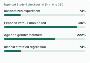
In Gordon et al.’s Study 4, the randomized checkout lift estimate was 73%, compared with 316% from an exposed-versus-unexposed comparison and 74% from the richest reported stratified regression. These are lift estimates for the same campaign, not checkout conversion rates.
Gordon et al., A Comparison of Approaches to Advertising Measurement
Why a near-zero experiment can disagree sharply with modeled lift
In Gordon et al.’s Study 9, randomized checkout lift was estimated at 2.4%, while the closest displayed observational estimate was 1,306%. The 2.4% result was reported as different from zero at the 10% level, and the finding is campaign-specific.
Gordon et al., A Comparison of Approaches to Advertising Measurement
How wide advertising ROI uncertainty can be
Lewis and Rao’s 2015 analysis of 25 randomized advertising experiments reported a median ROI interval over 100 percentage points wide. The median ROI standard error was 26.1 percentage points in retail experiments and 115 percentage points in brokerage experiments.
Lewis and Rao, The Unfavorable Economics of Measuring the Returns to Advertising
Advertising experiment size depends on the decision
In Lewis and Rao’s median-campaign calculation, distinguishing 50% ROI from break-even required about nine times the experiment size discussed at baseline. That multiple depends on the authors’ study economics and uncertainty, and is not a sample size rule for checkout recovery.
Lewis and Rao, The Unfavorable Economics of Measuring the Returns to Advertising
A narrower ROI decision can require far more data
In Lewis and Rao’s 2015 study, their idealized calculation put the median campaign at roughly nine times its original size to distinguish 50% ROI from break-even and 62 times for a 10% ROI difference. The comparison assumes additional independent person-weeks and is specific to those advertising economics.
Lewis and Rao, The Unfavorable Economics of Measuring the Returns to Advertising
Why large experiments can remain noisy
Lewis and Rao reported that each of their 25 advertising field experiments exceeded 500,000 unique users and most exceeded one million. Individual-level sales standard deviation was typically about ten times the mean over the evaluation window.
Lewis and Rao, The Unfavorable Economics of Measuring the Returns to Advertising
Break-even can move while the measured order gap stays fixed
In Take Rate’s worked example, $400 of treatment cost across 2,000 assigned shoppers breaks even at a 0.50-point order-rate gap with $40 contribution per additional order. At $24 contribution it takes approximately 0.83 points. These are illustrative calculations, separate from Lewis and Rao’s published experiments.
Lewis and Rao, The Unfavorable Economics of Measuring the Returns to Advertising
Four times the sample halves standard error under a stable variance model
Taking Lewis and Rao’s reported 26.1-point median retail ROI standard error as an illustrative starting value, four times the independent observations would reduce it to 13.05 points if variance per observation stayed constant.
Lewis and Rao, The Unfavorable Economics of Measuring the Returns to Advertising
Stratified and randomized estimates disagreed on sign in three checkout studies
In Gordon et al. Table 6, three of 14 checkout comparisons (21.43%) had opposite signs for the stratified observational and randomized lift point estimates. The affected rows were Studies 8, 10 and 15.
Gordon et al., A Comparison of Approaches to Advertising Measurement
Checkout comparisons in the authors’ 2019 experimental advertising paper. Count study rows with different signs and divide by the 14 checkout rows.
Study 8 retained a 35.9-point gap after stratification
In Gordon et al. Study 8, estimated checkout lift was +179% for exposed versus unexposed users, +33% after stratification and −2.9% in the randomized estimate. The latter two point estimates differed by 35.9 points.
Gordon et al., A Comparison of Approaches to Advertising Measurement
Study 8 checkout estimates from three methods in the same paper. Subtract the randomized estimate from the stratified estimate.
Compare the results
A larger dataset does not make two groups comparable
Gordon and colleagues studied 15 US Facebook advertising experiments comprising 500 million user-experiment observations and 1.6 billion ad impressions. They compared observational estimates with results from randomized designs. In seven of the 14 studies with a checkout outcome, the observational point estimates were consistently more than a factor of three off the randomized result. This is evidence about those studied methods and campaigns.
In Study 4, an exposed-versus-unexposed comparison suggested 316% checkout lift. Matching on age and gender brought it to 222%, while the experiment estimated 73%. The richest reported stratified regression was much closer at 74%. That is an important counterexample. Richer adjustment can work in a specific campaign. The same model choice cannot be assumed to work next time.
Study 9 shows the other side of that result. The randomized estimate was 2.4%, while the nearest observational estimate the authors reported was 1,306%. Only 6.6% were exposed in that study. The authors proposed this as one reason targeting could concentrate on unusually likely responders. They also describe Study 15, where almost every observational method underestimated lift. The correction is a more defensible comparison group, not a fixed discount applied to every attributed revenue claim.
Start with the decision threshold in orders or contribution
A merchant testing checkout recovery can set the threshold before reading the outcome. Suppose 2,000 eligible shoppers enter each arm, the control has 80 valid orders and the treatment has 100. That is 4% versus 5%, a gap of one percentage point. At a fixed $40 contribution per extra order and a $400 cost for treatment at that scale, the point estimate is $400 in additional contribution after cost.
The break-even threshold under those assumptions is 10 additional valid orders, or 0.50 percentage points over 2,000 treated shoppers. With independent customer-level assignments and a simple normal approximation, a 95% interval for the observed difference is approximately −0.29 to +2.29 percentage points. The point estimate clears the threshold while the interval spans it. The experiment leaves both profitable and unprofitable outcomes plausible.
If refunds, discounts and product mix matter, define contribution after those deductions before making the decision. The same extra-order count can have different economics depending on which products sold and which customers would have paid full price. Track contribution directly if the margin assumption is material. The worked numbers are hypothetical, and the arithmetic makes the decision rule visible.
The same point estimate can lead to a different decision
Keep the hypothetical control and treatment rates at 4% and 5%. With 10,000 independent shoppers per group, the approximate interval becomes +0.43 to +1.57 percentage points. With 20,000 per group, it becomes +0.59 to +1.41. If the cost and per-order contribution scale so the break-even gap remains 0.50 points, only the largest of these examples clears that threshold at its lower interval bound.
Lewis and Rao found a median ROI standard error of 26.1 percentage points for the retail subset of their advertising experiments, versus 115 for brokerage experiments. Their calculations illustrate why the economics and variance matter to precision. A smaller store can ask whether a longer valid window or a less noisy primary outcome would change the decision, and estimate the practical cost of waiting.
Use an analysis that matches the assignment. The simple interval in this example assumes independent shopper-level observations and one fixed comparison. Randomizing by region, repeatedly testing a running result, or placing repeat visits from one shopper in both arms changes that assumption. A causal result and a useful business decision both need the right unit.
Keep attribution, eligibility and program impact separate
Use the reporting system to understand which touchpoints it credited. Use the randomized group assignment for the rollout comparison. A buyer who already purchased before a scheduled reminder can remain in the group they were assigned to even though you correctly suppress the message. Removing that buyer because the send did not happen can recreate the selection problem the experiment was meant to solve.
Document the eligibility window, assignment unit, suppression policy, order validity rule and outcome cutoff. Check that both groups had equal opportunity for later orders and refunds to arrive. Report the assigned counts, order or contribution outcome, estimated gap, uncertainty interval and break-even threshold together. A statistically detectable improvement can still be too small to pay for the program.
Choose the smallest difference that would change the decision
Lewis and Rao observed that every trial included more than 500,000 unique users and most exceeded one million. Individual-level sales had a standard deviation typically about ten times their mean over the campaign evaluation window. This helps explain why large randomized samples could still leave wide uncertainty around returns.
Under their idealized calculation, adding independent person-weeks to the median campaign would take about nine times its size to distinguish 50% ROI from break-even and about 62 times its size to detect a 10% ROI difference at the intended power. The smaller decision threshold calls for much greater precision. Neither multiple transfers directly to a checkout program.
For an ecommerce test, write down the smallest contribution difference that would change the rollout. Set an analysis window and use historical order and refund variability to estimate whether the design has a realistic chance of distinguishing it. If the answer would be the same for effects on either side of the interval, a more precise result may add little to the decision. If the interval spans a material loss and a material gain, keep the uncertainty in the decision rather than presenting the positive midpoint alone.
A return-adjusted margin can change the rollout decision
Return to the worked example with 2,000 treated shoppers, 20 extra valid orders at the point estimate and $400 of cost. At $40 per extra order, break-even is 0.50 percentage points. If expected contribution per additional order falls to $24 after refunds, discount effects or product mix, break-even rises to about 0.83 points. Twenty additional orders at the lower margin would leave $80 after cost.
The randomized order counts have not changed. What changed is the commercial threshold. The same approximate interval around a one-point lift still spans the lower and higher thresholds. This is why the campaign can appear more or less attractive depending on a cost assumption even though the causal estimate is identical.
Where possible, define the paid-order and refund maturity rules before the test. Track contribution for both groups on the assignment denominator. If the cost and margin are uncertain, report a sensitivity range and show which range of effects would make the decision change. The arithmetic example is hypothetical; the Lewis and Rao evidence explains why enough precision to answer the economic question is difficult to obtain.
Translate uncertainty into the sample you would need
Before increasing spend to run an experiment, ask whether the larger test could actually settle the decision. Lewis and Rao report a median retail ROI standard error of 26.1 percentage points in their field experiments. This is a useful scale for thinking about noisy measurement, and a new program can have a very different variance.
In a worked example with independent observations and a stable outcome variance, quadrupling the sample halves the standard error. Starting at 26.1 points gives 13.05 points. A 20-point decision threshold moves from 0.77 to 1.53 standard errors away. The larger study is more precise. It can still leave a decision unresolved.
Start with recent outcomes for the population you can randomize. Use them to estimate how many purchases and how much contribution you normally see. Preserve customer or market clustering when estimating uncertainty. If the required sample is unrealistic, test a narrower eligibility policy or commit to a decision range before launch. Avoid raising budget solely because the first estimate looked promising.
A large adjustment can still reverse the decision
In Gordon and colleagues’ Table 6, the stratified observational estimate and randomized point estimate had opposite signs in three of 14 checkout studies. In two of them the observational adjustment suggested a loss while the experiment pointed up. In the third it suggested a gain while the experiment pointed down. The direction matters when a team is choosing whether to increase budget, cancel a program or run a more informative test.
Study 8 makes the distinction tangible. Exposed versus unexposed customers differed by +179% in the unadjusted comparison. Stratification brought the estimate down to +33%, closer to the randomized point estimate of −2.9%. The remaining distance was still 35.9 percentage points and the sign still differed. A method can reduce a large discrepancy and leave the business decision unresolved.
Treat the gap from break-even as the decision quantity
The same paper reports that six of 14 checkout experiments fell short of statistical significance at the 5% level. That is a separate property from whether the observational estimate points in the right direction. A randomized result may identify a credible comparison while leaving a broad range of economically plausible effects.
For a campaign with a fixed contribution target, write the break-even increment and plausible losses before looking at the results. Keep an observational estimate as a diagnostic for audience mix and delivery. Use the assigned groups to estimate the causal effect, then show the interval relative to the break-even target. If it spans both loss and a worthwhile gain, compare the value of learning with the cost of leaving the program on. A different channel or audience can need its own test even when the current campaign is conclusive.
A fair comparison can still leave the budget decision open
Your checkout recovery holdout ends and the treatment group spent more than the control group. The result looks promising. Before you expand the program, you need to know how much uncertainty is around that difference. A modest positive estimate can be consistent with a result below break-even and with one that would justify expanding.
Random assignment gives the comparison its force. Some shoppers would have finished their order without a reminder, and the holdout gives you a way to account for them. Precision is a separate issue. If purchase values vary widely or relatively few eligible shoppers order during the test, one period's result may leave a wide range of outcomes plausible.
What the 25 advertising experiments found
Randall Lewis and Justin Rao analyzed 25 randomized field experiments, including 19 for retailers and six for financial service firms. The campaigns represented about $2.8 million in digital advertising spend together. Across the experiments, the median confidence interval for return on investment was wider than 100 percentage points. The size of the campaigns is what makes the observation worth keeping in mind.
The paper reports a median ROI standard error of 26.1 percentage points for the retail experiments. A conventional normal approximation turns that standard error into an interval width of about 102 percentage points. That is a calculation from the study's reported standard error. A particular experiment can have a much narrower or wider interval, and a checkout recovery test has its own audience, costs and purchase patterns.
Put the break-even point next to the result
Choose an outcome before the pilot. For example, you might use incremental contribution per eligible shopper over a fixed period, with discounts, refunds and the relevant program costs treated consistently across the groups. Write down what would make a change worth operating. If your chosen measure already deducts the program cost, zero is break-even. You may still need a higher threshold to justify rollout work.
When the result comes in, put the threshold beside the estimate and its interval. An interval entirely above your threshold supports a different decision from one that stretches across it. An interval entirely below the threshold can be informative even if the program increased gross sales. The decision should follow the economics you wrote down for that test.
Check which shoppers the result represents
Say the program sends checkout reminders only to people who are eligible to receive them. Make that the starting audience. Then keep people in the groups they were assigned to, including anyone in treatment who never received a message. If you compare only shoppers whose message was delivered with everyone in the control, you risk comparing different populations. Delivery status can be useful for troubleshooting without becoming the basis for the lift claim.
Set the outcome window and assignment rules before seeing the sales. Check that you can trace refunds and store costs on the same basis for both groups. Where a few large orders can dominate the result, record the spread in order values as well as the total. Those details make the range of plausible outcomes easier to interpret and help you work out what a longer or larger test would need.
Write the conclusion somebody else could act on
Record who was eligible, what counted as an order, how long you observed outcomes, which costs you included and where the estimate sat relative to break-even. Keep the interval with the point estimate when you pass the result along. A teammate should be able to tell whether your conclusion concerns a particular channel, offer or checkout flow.
If the interval crosses the decision threshold, use the pilot to identify what would make another test informative. An unreliable link between orders and eligible shoppers is a measurement problem. A small eligible cohort or widely varying order values is a precision problem. Each suggests different work before the next decision. The original experiments are useful because they separate uncertainty from the fairness of the comparison.
Study data
| Measure | Value | Context |
|---|---|---|
| Randomized field experiments | 25 experiments | Paper reports 25 field experiments. |
| Retail field experiments | 19 experiments | Nineteen experiments were for retailers. |
| Financial-services field experiments | 6 experiments | Six experiments were for financial-service firms. |
| Combined advertising expenditure | About $2,800,000 | Published collective expenditure is approximately $2.8 million. |
| Median ROI confidence interval width | More than 100 percentage points | Published median ROI interval width exceeds 100 percentage points. |
| Median ROI standard error in retail experiments | 26.1 percentage points of ROI | Retail-experiment median ROI standard error is 26.1 percentage points. |
| Measure | Value | Context |
|---|---|---|
| Randomized US advertising experiments in the Gordon study | 15 experiments | Scope of the method comparison |
| User-experiment observations in the Gordon study | 500 million | Observations can repeat a user across experiments |
| Ad impressions in the Gordon study | 1.6 billion | Impressions are exposure events |
| Smallest Gordon campaign sample | 2 million users | Published range endpoint |
| Largest Gordon campaign sample | 140 million users | Published range endpoint |
| Checkout studies consistently off by more than a factor of three | 7 of 14 studies | Seven of the 14 checkout outcomes had observational point estimates consistently more than threefold off |
| Study 4, randomized checkout lift | 73% | Randomized experiment benchmark in that campaign |
| Study 4, exposed versus unexposed checkout lift | 316% | Observational comparison includes differences in who was exposed |
| Study 4, age-and-gender matched checkout lift | 222% | Observational match on age and gender only |
| Study 4, richest stratified regression checkout lift | 74% | Observational estimate reported next to the 73% experimental value |
| Study 9, randomized checkout lift | 2.4% | Reported as statistically different from zero at the 10% level |
| Study 9, closest observational checkout lift | 1,306% | Closest of the displayed observational estimates in that study |
| Study 9, share exposed to advertising | 6.6% | Authors propose low exposure as one possible explanation for the discrepancy |
| Study 15, stratified estimate | -13% | Rounded lift point estimate |
| Study 15, randomized estimate | 2.4% | Rounded lift point estimate |
| Study 10, stratified estimate | -15% | Rounded lift point estimate |
| Study 10, randomized estimate | 2% | Rounded lift point estimate |
| Study 8, stratified estimate | 33% | Rounded lift point estimate |
| Study 8, randomized estimate | -2.9% | Rounded lift point estimate |
| Measure | Value | Context |
|---|---|---|
| Median ROI standard error in financial-services studies | 115 percentage points of ROI | Median standard error for the financial-services subset |
| Sample-size multiplier to distinguish 50% ROI from break-even in their median scenario | 9 times | Scenario-specific sample multiple |
| Scale the authors say informative ad experiments can require | More than 10 million person-weeks | Potential experiment scale |
| Median campaign size multiplier to distinguish a 10% ROI difference | 62 times | Illustrative power calculation reported by the authors |
| Smallest unique-user scale exceeded by every trial | More than 500000 users | Each trial exceeded 500,000 unique users |
| Unique-user scale exceeded by most trials | More than 1000000 users | Most trials exceeded one million unique users |
| Typical individual-level sales standard deviation relative to mean | 10 times | Authors’ description of purchase-value variation |
What changes when you compare the figures
| Comparison | Result | Calculation |
|---|---|---|
| Illustrative normal-approximation 95% interval width at that retail median standard error | 102.312 percentage points | = 2 × 1.96 × standard error |
| Study 4 exposed comparison minus randomized estimate | 243 percentage points | = 316 − 73 |
| Study 4 matched comparison minus randomized estimate | 149 percentage points | = 222 − 73 |
| Study 4 richest stratified estimate minus randomized estimate | 1 percentage points | = 74 − 73 |
| Study 9 closest observational estimate minus randomized estimate | 1,303.6 percentage points | = 1,306 − 2.4 |
| Share of checkout studies with consistent more-than-threefold discrepancies | 50% | = 7 ÷ 14 × 100 |
| Financial-services to retail median ROI standard error ratio | 4.41 times | = 115 ÷ 26.1 |
| Median 10% ROI discrimination multiplier divided by the 50% comparison multiplier | 6.89 times | = 62 / 9 |
| Hypothetical break-even gap at $40 contribution per order | 0.5 percentage points | = 400 / 40 / 2000 * 100 |
| Hypothetical break-even gap at $24 contribution per order | 0.83 percentage points | = 400 / 24 / 2000 * 100 |
| Hypothetical net contribution at 20 additional orders and $24 each | $80.00 | = 20 * 24 - 400 |
| Illustration, standard error at four times the sample | 13.05 percentage points | = 26.1 / 2 |
| Illustration, standardized effect for a 20-point ROI difference | 0.77 standard errors | = 20 / 26.1 |
| Illustration, standardized effect after quadrupling the sample | 1.53 standard errors | = 20 / 13.05 |
| Share of checkout studies with a sign reversal | 21.429% | = 3 / 14 * 100 |
| Study 8, remaining difference after stratification | 35.9 percentage points | = 33 - (-2.9) |
| Study 8, original exposed-to-randomized difference | 181.9 percentage points | = 179 - (-2.9) |
| Share of checkout studies short of 5% significance | 42.857% | = 6 / 14 * 100 |
Methodology and sources
Study figures come from the final 2015 Quarterly Journal of Economics article. The example interval width multiplies the published retail median standard error by twice 1.96, using a normal approximation. It describes the order of magnitude of the original results and gives no estimate for a specific store or recovery channel.
We transcribed Gordon et al.’s sample scope, Section 7.2 cases and Figure 10 comparisons, and Lewis and Rao’s 2015 results for advertising ROI precision. Observational and experimental lift estimates share a campaign outcome in the selected examples. Results from the two papers do not share an outcome or base and are kept separate. The worked checkout examples use independent two-group binomial estimates: standard error is the square root of the sum of p × (1 − p) divided by group size for each arm. The approximate 95% bounds add and subtract 1.96 standard errors from the difference in rates. The CSV reports hypothetical counts and a 0.50 percentage-point threshold to show how the decision changes with precision.
Download the source data (CSV)
Download the calculations (CSV)
Download the citation notes (CSV)
Related reading
Sample ratio mismatch statistics for checkout A/B tests
A/B test peeking statistics for checkout experiments
Sources and definitions
The Unfavorable Economics of Measuring the Returns to Advertising
Gordon et al., A Comparison of Approaches to Advertising Measurement
The source data includes the population, period, denominator and limitations for every figure.