


Quick answer
In a public randomized retail email test, the men’s merchandise email produced 76.59 additional visitors and 6.81 additional buyers per 1,000 customers assigned, compared with no email. Recorded spend rose by about $0.77 per assigned customer over two weeks. Evaluate the result you need for rollout, using everyone assigned to the campaign or holdout.
Kevin Hillstrom, MineThatData Email Analytics and Data Mining Challenge · hillstorm1.s3.us-east-2.amazonaws.com
Key findings and sources
One email added 76.59 visitors and 6.81 buyers per 1,000
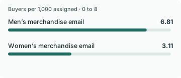
In Take Rate’s reanalysis of Kevin Hillstrom’s 64,000-customer randomized email dataset, the men’s merchandise email added 76.59 visitors and 6.81 buyers per 1,000 assigned versus no email over two weeks.
Kevin Hillstrom, MineThatData Email Analytics and Data Mining Challenge · hillstorm1.s3.us-east-2.amazonaws.com
The other email had a smaller purchase contrast
In the same randomized dataset, the women’s merchandise email added 45.23 visitors and 3.11 buyers per 1,000 assigned versus no email over two weeks. All rates use the full randomized arm.
Kevin Hillstrom, MineThatData Email Analytics and Data Mining Challenge · hillstorm1.s3.us-east-2.amazonaws.com
Observed spend increased by different amounts by campaign
In the Hillstrom dataset, two-week spend per assigned customer was $0.65 for no email, $1.08 for the women’s merchandise email and $1.42 for the men’s merchandise email. These are recorded spend figures before a margin adjustment.
Kevin Hillstrom, MineThatData Email Analytics and Data Mining Challenge · hillstorm1.s3.us-east-2.amazonaws.com
Purchases also occurred in the holdout
In the Hillstrom no-email arm, 122 of 21,306 assigned customers purchased within two weeks. This 0.57% baseline is part of the randomized comparison.
Kevin Hillstrom, MineThatData Email Analytics and Data Mining Challenge · hillstorm1.s3.us-east-2.amazonaws.com
Email purchase lift was similar across two pre-assignment recency bands
In the historical Hillstrom experiment, the men’s merchandise email added 7.33 buyers per 1,000 assigned among one-to-three-month buyers and 7.29 among seven-to-12-month buyers, each against its own no-email arm.
Kevin Hillstrom, MineThatData Email Analytics and Data Mining Challenge
Two-week outcomes after randomized assignment, split using prior purchase recency. Subtract the control purchase proportion from the treatment purchase proportion within each recency band.
The recency difference was smaller than its sampling uncertainty
The observed difference between the two recency-band purchase lifts was 0.04 buyers per 1,000. An unadjusted approximate 95% interval was -4.27 to 4.35 buyers per 1,000.
Kevin Hillstrom, MineThatData Email Analytics and Data Mining Challenge
Two disjoint post-hoc recency bands from Hillstrom’s historic randomized retail experiment. Use the sum of the independent binomial variances across the four cells and a 1.96 standard-error interval.
Compare the results
Start with the outcome that decides the rollout
A report can look strong on traffic and modest on paid orders at the same time. These counts tell you where the effect appears in the funnel. Each uses the same eligible customer group, so you can compare the two without narrowing the analysis to people who clicked or visited.
The original challenge randomly assigned customers to a men’s merchandise email, a women’s merchandise email or no email. Those are campaign labels. They do not identify the customer’s gender. The no-email customers could still visit and buy, which is exactly the background activity the test needs to measure.
Put the visit and purchase differences on one scale
The men’s merchandise email added 76.59 visitors and 6.81 buyers per 1,000 assigned. The women’s merchandise email added 45.23 visitors and 3.11 buyers per 1,000 assigned. The campaigns differed in their observed effects. These figures also show why the visit count is a poor stand-in for the number of additional orders.
Dividing incremental purchases by incremental visits does not recover a conversion rate for the people persuaded to visit. The data do not identify who would have visited anyway, and the email can change what a customer does after arriving. Keep each contrast on the assignment denominator.
Translate spend into a decision the merchant can use
Average recorded spend was about $0.65 with no email, $1.08 for the women’s merchandise email and $1.42 for the men’s merchandise email. That is revenue before any adjustment for contribution margin, fulfillment cost or later returns. A merchant can define an outcome that deducts those costs and compare the groups on that measure.
For a recovery program, predefine who could be contacted and the period during which a completed order counts. Record every assigned customer, including people who buy before the message reaches them. Read visits alongside purchases so the team can see whether a change helped more people return, helped them complete the order, or both.
Both recency groups benefited in the point estimate
For customers who had last purchased one to three months earlier, the men’s merchandise email added 7.33 buyers per 1,000 assigned compared with no email. For customers last purchasing seven to 12 months earlier, it added 7.29. These are pre-assignment groups. The outcome still includes every assigned customer inside the group, including people who never visited the site.
The point estimates differ by 0.04 buyers per 1,000. A simple large-sample comparison of those two unadjusted lift estimates gives an approximate 95% interval of -4.27 to 4.35 buyers per 1,000 for the difference. The interval includes zero and materially different policies in either direction. It offers little reason to choose a recency policy just because one rounded point estimate is higher.
A different natural purchase rate can still support the same message policy
A team may see more purchases among recent buyers after a message. That alone is a reason to look at the group’s natural purchase rate. In this data, recent buyers had a higher no-email purchase rate than buyers whose last purchase was seven to 12 months earlier. Each campaign effect therefore needs its own group’s no-email comparison.
Preselect a recency band where treatment rules genuinely differ, such as a replenishment window or a recent complaint. Verify enough assigned buyers and recorded orders in each band before asking which policy won. Evaluate cost and customer experience within that band. If uncertainty spans both choices, keep a stable policy and run a separate confirmation where the actual decision is whether, or when, to contact those customers.
Study data
| Measure | Value | Context |
|---|---|---|
| No email, assigned customers | 21,306 customers | Original aggregation, assignment denominator |
| No email, site visitors | 2,262 customers | Original aggregation, assignment denominator |
| No email, buyers | 122 customers | Original aggregation, assignment denominator |
| No email, recorded spend | $13,908.33 | Original aggregation, assignment denominator |
| No email, visit rate | 10.61673% | Original aggregation, assignment denominator |
| No email, purchase rate | 0.57261% | Original aggregation, assignment denominator |
| No email, spend per assigned customer | 0.65279 USD per customer | Original aggregation, assignment denominator |
| Men’s merchandise email, assigned customers | 21,307 customers | Original aggregation, assignment denominator |
| Men’s merchandise email, site visitors | 3,894 customers | Original aggregation, assignment denominator |
| Men’s merchandise email, buyers | 267 customers | Original aggregation, assignment denominator |
| Men’s merchandise email, recorded spend | $30,311.69 | Original aggregation, assignment denominator |
| Men’s merchandise email, visit rate | 18.27568% | Original aggregation, assignment denominator |
| Men’s merchandise email, purchase rate | 1.25311% | Original aggregation, assignment denominator |
| Men’s merchandise email, spend per assigned customer | 1.42262 USD per customer | Original aggregation, assignment denominator |
| Men’s merchandise email, additional buyers per 1,000 | 6.81 buyers per 1,000 assigned | Two-week randomized assignment difference |
| Women’s merchandise email, assigned customers | 21,387 customers | Original aggregation, assignment denominator |
| Women’s merchandise email, site visitors | 3,238 customers | Original aggregation, assignment denominator |
| Women’s merchandise email, buyers | 189 customers | Original aggregation, assignment denominator |
| Women’s merchandise email, recorded spend | $23,038.11 | Original aggregation, assignment denominator |
| Women’s merchandise email, visit rate | 15.14004% | Original aggregation, assignment denominator |
| Women’s merchandise email, purchase rate | 0.88371% | Original aggregation, assignment denominator |
| Women’s merchandise email, spend per assigned customer | 1.0772 USD per customer | Original aggregation, assignment denominator |
| Women’s merchandise email, additional buyers per 1,000 | 3.11 buyers per 1,000 assigned | Two-week randomized assignment difference |
What changes when you compare the figures
| Comparison | Result | Calculation |
|---|---|---|
| Men’s merchandise email, additional visitors per 1,000 | 76.59 visitors per 1,000 assigned | = (3894 / 21307 - 2262 / 21306) * 1000 |
| Men’s merchandise email, additional buyers per 1,000 | 6.81 buyers per 1,000 assigned | = (267 / 21307 - 122 / 21306) * 1000 |
| Men’s merchandise email, additional spend per assigned customer | 0.77 USD per customer | = (30311.69 / 21307 - 13908.33 / 21306) * 1 |
| Women’s merchandise email, additional visitors per 1,000 | 45.23 visitors per 1,000 assigned | = (3238 / 21387 - 2262 / 21306) * 1000 |
| Women’s merchandise email, additional buyers per 1,000 | 3.11 buyers per 1,000 assigned | = (189 / 21387 - 122 / 21306) * 1000 |
| Women’s merchandise email, additional spend per assigned customer | 0.42 USD per customer | = (23038.11 / 21387 - 13908.33 / 21306) * 1 |
| Women’s merchandise email, dollars per 1,000 assignments | 424.41 USD per 1,000 assigned | = (23038.11 / 21387 - 13908.33 / 21306) * 1000 |
| One-to-three-month buyer lift per 1,000 | 7.326 buyers per 1,000 assigned | = (122 / 7469 - 67 / 7438) * 1000 |
| Seven-to-12-month buyer lift per 1,000 | 7.289 buyers per 1,000 assigned | = (96 / 9165 - 29 / 9102) * 1000 |
| Difference between purchase lifts in two recency bands | 0.038 buyers per 1,000 assigned | = (122 / 7469 - 67 / 7438 - 96 / 9165 + 29 / 9102) * 1000 |
| Approximate contrast standard error | 2.198 buyers per 1,000 assigned | = ((122/7469)*(1-122/7469)/7469 + (67/7438)*(1-67/7438)/7438 + (96/9165)*(1-96/9165)/9165 + (29/9102)*(1-29/9102)/9102)**0.5 * 1000 |
Methodology and sources
Group the 64,000 public rows by randomized email assignment. Sum visit, conversion and spend. Divide every outcome by all customers assigned to that arm. Subtract the no-email rate for a treatment contrast. The packaged source archive was verified against its published MD5 and the reproducible script records a SHA-256. The dataset measures visits rather than email clicks. Figures describe existing customers at one historical retailer.
Download the source data (CSV)
Download the calculations (CSV)
Download the citation notes (CSV)
Download the reproducible analysis script
Related reading
Incremental advertising return statistics and what a holdout can tell you
Sample ratio mismatch statistics for checkout A/B tests
Sources and definitions
Kevin Hillstrom, MineThatData Email Analytics and Data Mining Challenge
The source data includes the population, period, denominator and limitations for every figure.