


Quick answer
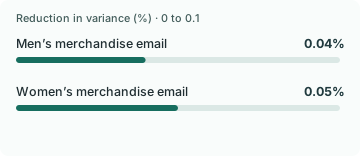
Past spend explained very little in this public retail test. An adjustment fitted on 32,000 customers reduced the estimated variance of two email-versus-control spend comparisons by 0.04% and 0.05% in the other 32,000 customers. Check how well your baseline measure predicts the outcome before counting on a smaller holdout.
Kevin Hillstrom, MineThatData Email Analytics and Data Mining Challenge · hillstorm1.s3.us-east-2.amazonaws.com
Key findings and sources
Prior and follow-up spend had a 0.00965 training correlation
Take Rate’s split of Hillstrom’s randomized retail email dataset found a Pearson correlation of 0.00965 between prior spend and two-week spend in the 32,000-row training half.
Kevin Hillstrom, MineThatData Email Analytics and Data Mining Challenge · hillstorm1.s3.us-east-2.amazonaws.com
64,000 customers in Hillstrom’s randomized retail email dataset, two weeks of outcomes Calculate Pearson correlation of history and spend in the even-indexed records.
The men’s email contrast lost 0.04% of estimated variance
In the held-out half of the Hillstrom dataset, a prior-spend adjustment fitted on separate records reduced estimated variance of the men’s merchandise email versus no-email spend contrast by 0.04%.
Kevin Hillstrom, MineThatData Email Analytics and Data Mining Challenge · hillstorm1.s3.us-east-2.amazonaws.com
64,000 customers in Hillstrom’s randomized retail email dataset, two weeks of outcomes Compare the raw and adjusted difference-in-means variance estimates on odd-indexed rows.
The women’s email contrast lost 0.05% of estimated variance
Using the same split and prior-spend adjustment, estimated variance for the women’s merchandise email versus no-email spend contrast fell 0.05% in the held-out rows.
Kevin Hillstrom, MineThatData Email Analytics and Data Mining Challenge · hillstorm1.s3.us-east-2.amazonaws.com
64,000 customers in Hillstrom’s randomized retail email dataset, two weeks of outcomes Compare estimated variance before and after adjustment for this arm and the shared control.
Both estimates used the same 10,720 held-out control customers
The held-out Hillstrom split contained 10,720 no-email customers, 10,529 assigned to the men’s merchandise email and 10,751 assigned to the women’s merchandise email. Spend comparisons included every customer in each evaluated arm.
Kevin Hillstrom, MineThatData Email Analytics and Data Mining Challenge · hillstorm1.s3.us-east-2.amazonaws.com
64,000 customers in Hillstrom’s randomized retail email dataset, two weeks of outcomes Count the assignment labels on odd-indexed rows in the public CSV.
Compare the results
Past purchases gave this experiment little leverage
Customers who spend more in the past sometimes spend more after assignment, which gives an experiment a way to reduce noise. In this dataset, the training correlation between past spend and the recorded two-week outcome was 0.00965. That is why the adjustment moved the estimate of variance so little in the untouched evaluation rows.
For the men’s merchandise email, the raw standard error was $0.2395 per assigned customer and the adjusted standard error was $0.2395 at the same precision. The variance reduction was 0.04%. The other campaign gave a 0.05% reduction against the same control. These figures come from a single split and describe the adjustment that was actually tested.
Check prediction before planning around an efficiency gain
The last 12 months of spend can have a weak connection with spend in the next two weeks. Store seasonality, customer tenure and long gaps between orders can all change that relationship. Try a relevant baseline such as comparable recent purchase days, or a pre-assignment checkout amount when that field is measured consistently across the eligible population.
Use earlier data to choose the measure. Freeze its definition and the adjustment before reading outcomes from the rollout test. If the original variable is missing for guests or new customers, specify how the experiment will handle that group and check the data coverage by arm. A post-message visit or reply would be caused by assignment and belongs outside the baseline.
Keep a revenue holdout interpretable at checkout
In this analysis, outcomes include all assigned customers, so people with no purchase contribute zero spend. Keep that rule when looking at checkout recovery. Conditioning on a reply or a return visit can change which customers appear in the two groups.
For a real decision, show both raw and adjusted results on a common denominator and preselect the estimate that determines rollout. Choose a follow-up period that can capture orders and returns. If prior data add little precision, plan the necessary audience and duration around the outcome variance you can actually observe.
Study data
| Measure | Value | Context |
|---|---|---|
| Training rows | 32,000 customers | Deterministic split |
| Training spend correlation | 0.009649 correlation | Original Pearson correlation |
| Training adjustment coefficient | 0.00050735 USD per USD | Original covariance-to-variance ratio |
| Men’s merchandise email raw difference | 1.0833603 USD per customer | Original out-of-sample contrast |
| Men’s merchandise email raw variance | 0.0573683 USD squared per customer squared | Original out-of-sample contrast |
| Men’s merchandise email adjusted difference | 1.0835609 USD per customer | Original out-of-sample contrast |
| Men’s merchandise email adjusted variance | 0.0573474 USD squared per customer squared | Original out-of-sample contrast |
| Men’s merchandise email variance reduction | 0.04% | Original variance ratio |
| Women’s merchandise email raw difference | 0.2627274 USD per customer | Original out-of-sample contrast |
| Women’s merchandise email raw variance | 0.0347965 USD squared per customer squared | Original out-of-sample contrast |
| Women’s merchandise email adjusted difference | 0.2618173 USD per customer | Original out-of-sample contrast |
| Women’s merchandise email adjusted variance | 0.034779 USD squared per customer squared | Original out-of-sample contrast |
| Women’s merchandise email variance reduction | 0.05% | Original variance ratio |
| Held-out control customers | 10,720 customers | Original split count |
What changes when you compare the figures
| Comparison | Result | Calculation |
|---|---|---|
| Men’s merchandise email variance reduction | 0.04% | = (1 - 0.057347396618 / 0.057368297849) * 100 |
| Men’s merchandise email unadjusted standard error | 0.2395 USD per customer | = 0.057368297849**0.5 |
| Men’s merchandise email adjusted standard error | 0.2395 USD per customer | = 0.057347396618**0.5 |
| Women’s merchandise email variance reduction | 0.05% | = (1 - 0.034778989463 / 0.034796458116) * 100 |
| Women’s merchandise email unadjusted standard error | 0.1865 USD per customer | = 0.034796458116**0.5 |
| Women’s merchandise email adjusted standard error | 0.1865 USD per customer | = 0.034778989463**0.5 |
Methodology and sources
Preserve source row order. Fit the slope of two-week spend on prior spend using the 32,000 even-indexed rows, pooled over the randomized arms. For each odd-indexed row, subtract the slope times its prior spend minus training mean prior spend. Compare each email arm with the same no-email control. Estimated variance of a difference in means is the sum of each arm’s sample variance divided by its customer count. Reduction is one minus adjusted variance divided by raw variance. This single deterministic split illustrates a precision check. Its effects can differ from the full-sample effects.
Download the source data (CSV)
Download the calculations (CSV)
Download the citation notes (CSV)
Related reading
Incremental advertising return statistics and what a holdout can tell you
Sample ratio mismatch statistics for checkout A/B tests
A/B test peeking statistics for checkout experiments
Sources and definitions
Kevin Hillstrom, MineThatData Email Analytics and Data Mining Challenge
The source data includes the population, period, denominator and limitations for every figure.